GOES-16 Color Animation with Python

Click on the image above to see the video in action!

Another GOES Animation

In a previous post, I wrote up a process for creating time-lapse animations of GOES-16 satellite imagery. However, the images I was using were from a heavily post-processed imagery product called GeoColor.

While I like the color processing and night-time cloud/light effects of these images, I wanted to try my hand at image processing techniques and work with raw satellite sensor data.

GOES on AWS and Processing netCDF Files

From my research on references for Earth observation imagery, I knew my starting point would be GOES on AWS. This is a free, publicly available data set where GOES satellite images are available via AWS S3 buckets in netCDF file format. I also decided to use Python for this project, relying on boto3 for accessing AWS S3 buckets, netCDF4 for manipulating netCDF files and PILLOW for image processing.

The GOES satellite has images available in 16 different bands at 15 min intervals, so I wrote up a Python script that gets a list of available image files in an S3 bucket for a given day of interest, and then downloads those files locally.

I also heavily relied on the work process described in this very helpful post on image processing netCDF files from GOES-16.

Generating True Color Images and Correcting Bad Pixels

While the GOES-R satellites have 16 bands of multi-spectral image data available, it does not have a true “green” spectral band. This means that true color imaging is not possible directly, so you need to do a little extra work.

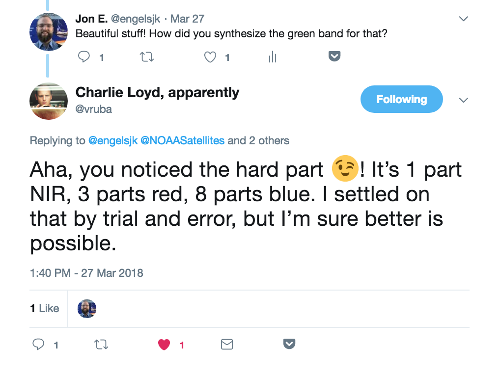
I asked Charlie Lloyd, a satellite imaging specialist at Mapbox, for tips on how he recreated a green band in his own true color GOES animation.

Using this info as a starting point, I wrote up a Python script to run through the following process:

• Query the GOES S3 bucket for files from a specific day/time.
• Download netCDF files from that day/time for each sensor band of interest.
• Convert radiance data from netCDF files into reflectance.
• Use the Blue, Red and Near IR channels to create a “Green” channel.
• Combine the Red, Green and Blue images to generate a true color RGB image.

The GOES-16 imager captures full disk images at 15 minute intervals, so this process repeated 96 times to generate true color images for one 24 hour period.

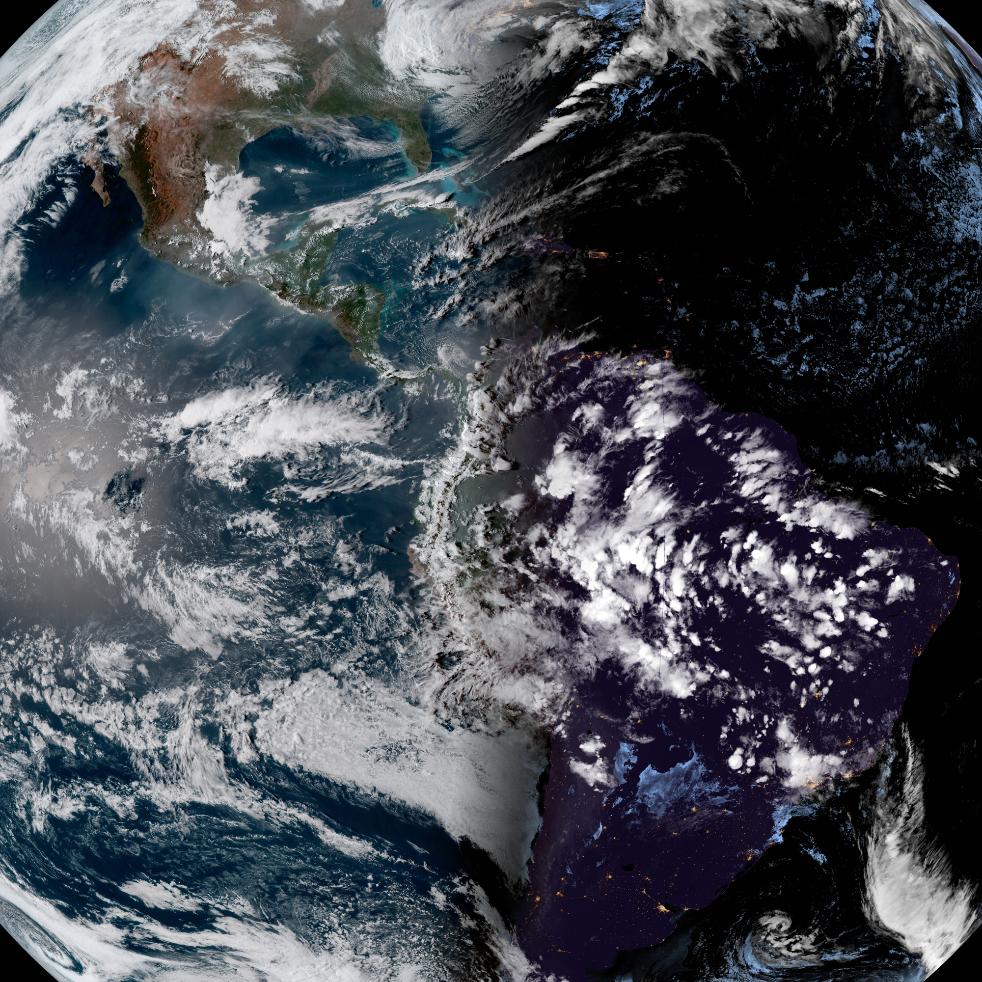
After successfully running through a number of images with this process, I discovered some issues with bad pixels at the edge of the Earth full disk during high sun angles.

In order to create a true color image, you need to combine Red, Green and Blue (or RGB) images. And in my case, to create the Green image, I needed to combine Red, Blue and Near IR images. But if you have enough bad pixels in those different image channels, then you’re also going to have bad pixels in the synthesized Green channel. And then your true color image will have artifacts like those in the image above, with either fully black pixels (i.e. no good pixels in any channel) or pixels that are missing one of the RGB components or have unbalanced values.

Needing a way to look into this in more detail, I saved grayscale images of each of the first 4 sensor bands so I could clearly see the problem.

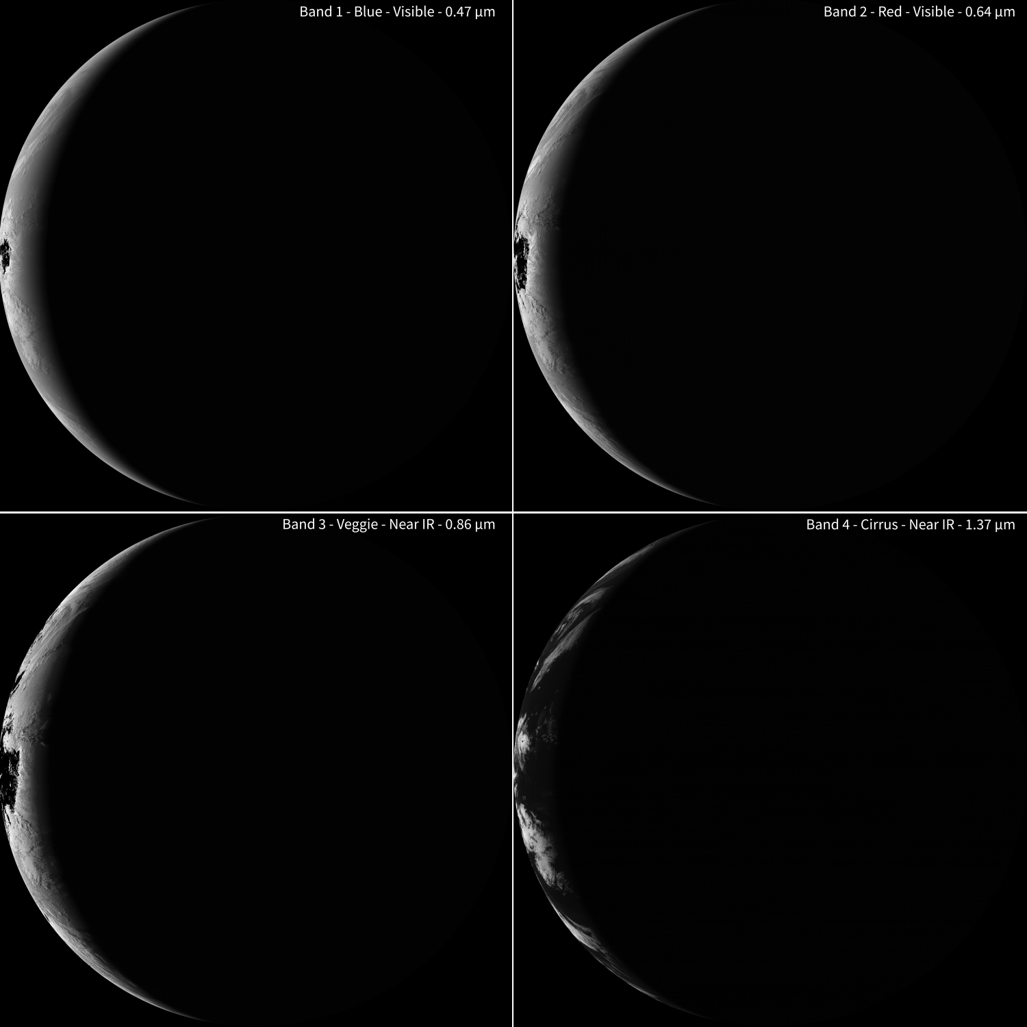
I’m still not sure the cause of these bad pixels (possible sensor saturation?) that show up black in each of the different sensor bands, but I needed a way to at least fake my way through fixing those pixels.

After a good bit of trial and error, I settled on a two-step process of pixel correction. The first step was to sequentially step through each Band 1-4 and use a linear regression fit (w/ ordinary least squares model) to relate each band to the other three bands, for all valid pixels in each image. Then I used that model to estimate values for every invalid pixel in each band. The second step was to then use the Red channel pixel values and set the Blue and Near IR pixel values for any bad pixel that wasn’t corrected in the first step.

I was surprised by the results of this correction process, particularly how many bad pixels I was able to recreate with the linear regression fit. I wasn’t particularly happy with the second step as it resulted in some areas with very flat white looking pixels, but it works well enough when needed (i.e. really high sun glint regions).

Final Results

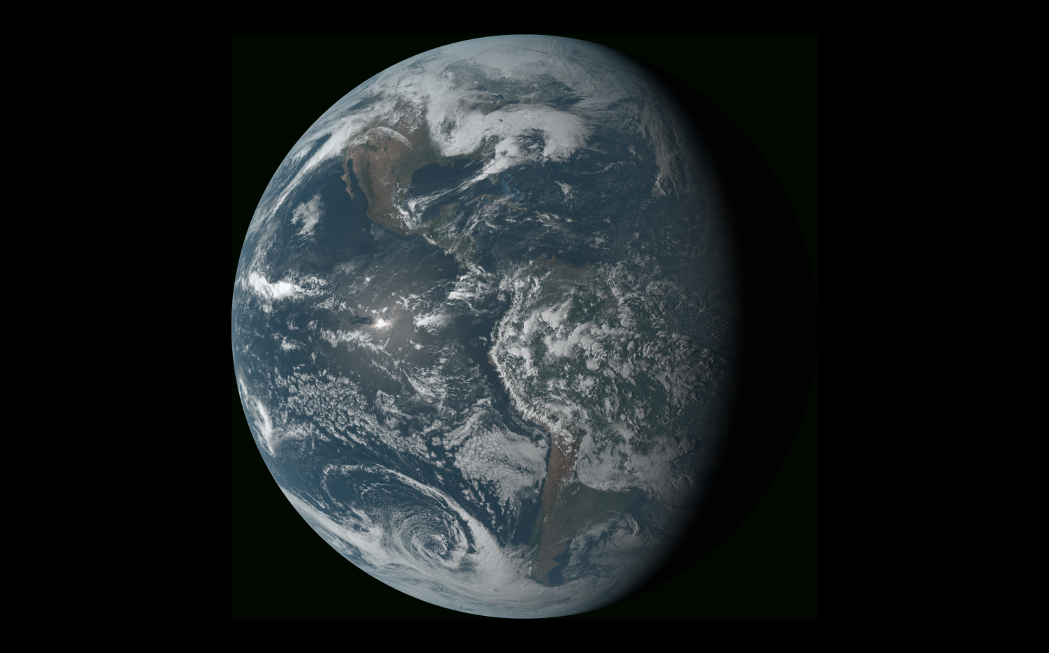
Overall, this process produced relatively clean true color imagery.

As expected, the colors are a bit muted by Rayleigh scattering since I didn’t do any atmospheric correction in the image processing steps. This could have been done by either a true Rayleigh scattering correction on the reflectance data (accounting for satellite and solar zeniths, atmospheric estimates, etc) or just an image color balance adjustment. I might revisit this work at some point to incorporate these corrections and make the colors pop a bit more!